Research
Generating a framework for interpreting and creating site specific responses using machine learning : Housing as a case

Primary Reaseacher
Guide: K.R. Machuchand
Rhinoceros + Grasshopper, Predictions using Python + Seaborn + Tensorflow

Motivations

The paper here is motivated by the bachelor’s thesis written in 2018, “BUILDING v/s building, an exploration in transient architecture; Case: Public health”. The criticism of the thesis revolves around the fact that the circulation and hierarchy of spaces are baked into the framework generating the floorplans. The solution although acceptable for a narrow view of application and typologies, lacks a degree of generalization and variance in terms of spatial planning. The intention is to generalize the problem and extrapolate the learnings made in the thesis to further a more general framework to build upon in the future.

Introduction

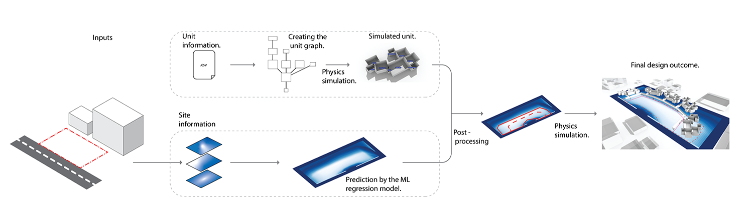
Design is seen as a decision-making process for a given circumstance which often deals with both logical reasoning and experience. The proposed framework aims to emulate the process of picking up design goals which are not programmed but arise from training (or ‘experience’), as a mixed approach between generative and learnt examples, with the use of machine learning methods such as stochastic gradient descent (SGD) regressors and deep neural networks (DNNs). Using housing as a premise, this framework has been tested, creating an output that exhibits implicit design goals of housing examples, with the use of graph structures (to create the housing units) and dynamic physics system (to drive the unit creation process). Our results point to the fact that given enough variety of balanced examples, a machine learning model can pick up on abstract design goals and recreate them contextually.

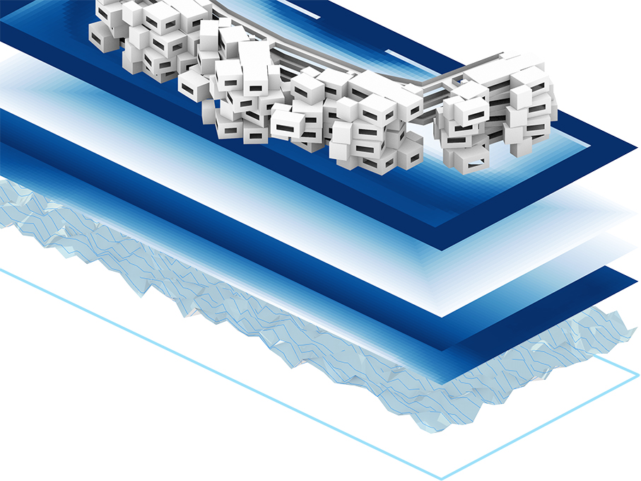
The overall framework is based on the premise that most mass housing is based on a certain floor plan shape which is dictated by circulation. Here we use a physics system to create a unit, then a machine learning system to create a floorplan ‘shape’ out of which a major artery is extracted and established. Lastly the artery is used to simulate the units (again using the physics system) to get the final building.

Unit generation

Generating a layout

Creating the units has two main components, drawing out the units and then packing them. The process of drawing out the units is as follows :

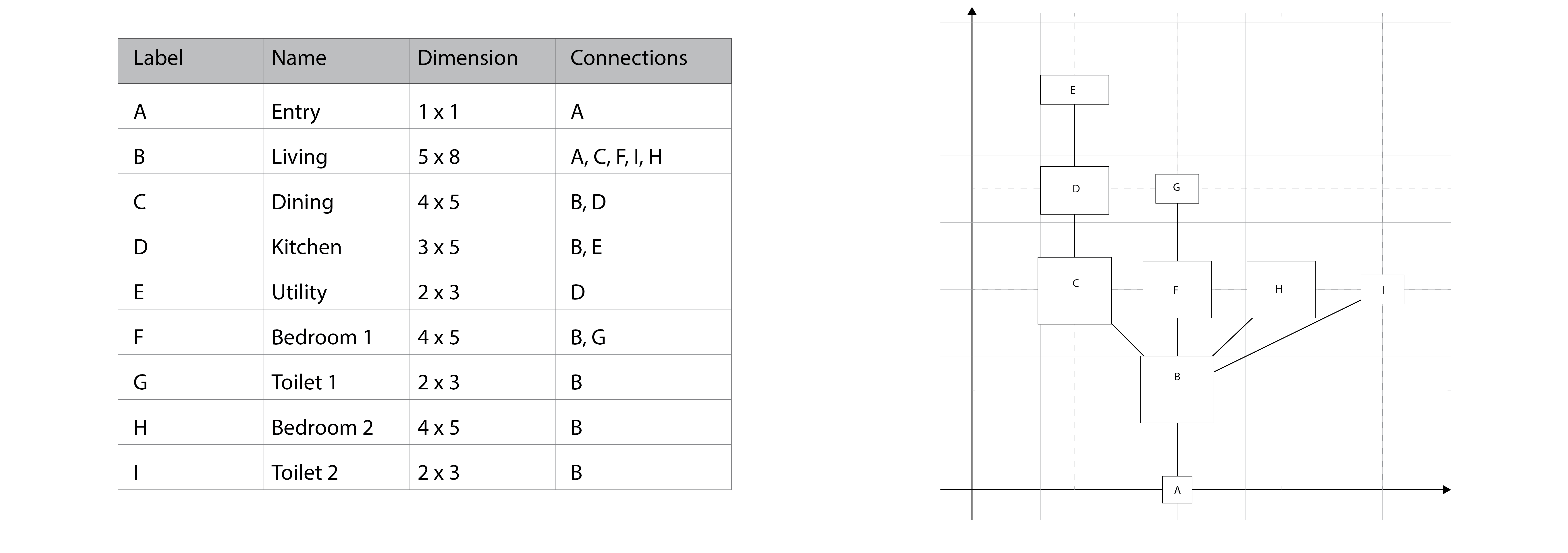
• Unit data is a set of information (Table 1) prepared beforehand
• The ‘pass’ through the objects starts at the “entry” using a Breadth First Search system
• A separate “drawing” class stores the graph information regarding the final diagram to be produced (The positions)
• The second ‘pass’ draws out the space at the position specified in the “drawing” class
• The final ‘pass’ draws out the connectors

The physics simulation

The notion of physical systems finding a point of equilibrium is the key idea used here to pack the spaces together this is leveraged so :

• The spatial graph generated from the tabulated data is to be simulated as a physical system to be in equilibrium
• The connectors are elements, simulated as per Sample Unit Data table. If a space is connected to multiple different spaces each connection is given the same degree of importance.
• The simulation of the edges connecting the vertices yields a better solution.
• The result of the simulation is a single unit

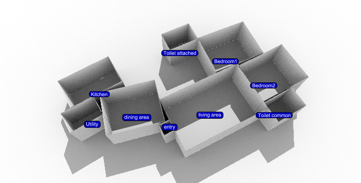
Summary of the process

Creating input vector for learning

The following graphic summarizes the process by which the Deep Neural Network makes a prediction. A key idea to be noted here is that the prediction made here is a logistic regression where the networks assigns a value between 0 and 1, in increments of 0.01. This allows the solution to be fine tuned based on the users requirement and to either narrow or expand the number of generated designs.
The attributes for learning are broken down into multiple layers of information, namely the solar radiation information, distance to site edge and distance to the access road. The model evaluates each part on the site with respect to these primary attributes and makes the prediction between 0 and 1. where values closer to 0 are fitter for consideration as opposed to 1 which are the worst. A part doesn’t alone influence the fitness as it does not address contextuality. Hence a window (array of neighboring parts) must be fed into the model for contextual information. At the same time there must be overall site information to be fed, such that the model recognizes the site as an overall ‘larger picture’.

Training data

The creation of a design is broken down into two distinct inputs which are not necessarily co-related to each other. The inputs being a site and the second being the design program and the two are treated independently. For each combination of site and design program there would be a single design solution which is generated by a human and thus there are certain biases which creep into the data and training samples. In this case, consciously the northern façade has been lengthened and U-shaped configuration facing the road are created as an implicit design goal, to test if the prediction model can perceive them. The granularity of dividing up the site is critical to artificially inflating the dataset for the training process. In this case; 10 sites (0.85 to 1.45 acres), 5 area programs, resulting in a total of 50 design solutions. In terms of raw samples, the sites are divided into 1x1 square meter grids. Thus the cumulative dataset is close to 230,860 samples which are randomized for training.

The Machine Learning framework

Trails with Stochastic Gradient Descent (S.G.D.)

Scikit-learn’s library of machine learning algorithms is useful for establishing a base for approximating what method of prediction would seem to do well. The SGD regressor is used to test whether the dataset is learnable or not. The result from this test is then used as a baseline for further exploration.

The Deep Learning framework

The results from deep learning experiments

First a model pool of 28 models with several hidden layers varying from 1 to 3 and a number of nodes varying from 32 to 256 were created. Of these 28 models the ones, which cross an out of sample validation accuracy of 65% after 15 epochs, were chosen for further training. The comparative analysis of all the model architectures (the format being – layer 1, layer 2, ... layer N) chosen are shown in the image below

Comparitive analysis Window Size or Downsample Size

Lastly as a point of enquiry. How does changing the ratio of the window size and the down-sample size affect the predictions. A variance of window and down-sample sizes were used to check which performed the best. The naming convention followed here is (A x B) where A is a integer number representing a square window for the window size and B is the down-sample size. Hence a 5 x 17 would mean a window size of 5 x 5 and a down-sample size of 17 x 17. The range of testing varied from a window dimension of 5 x 5 to 19 x 19 (intermediate values such as 7 X 11 etc. are accounted for. Only odd numbers can be used since there has to always be a central point around which we take a ‘swatch’ of data) whilst keeping the DNN model that we tested from the previous section the same.

What we found is that:

• Smaller window and down-sample sizes yield better results.
• The window size seems to be far more important to the accuracy of prediction than the down-sample size. Out hypothesis here is that the down-sample data is primarily interpreted as noise.

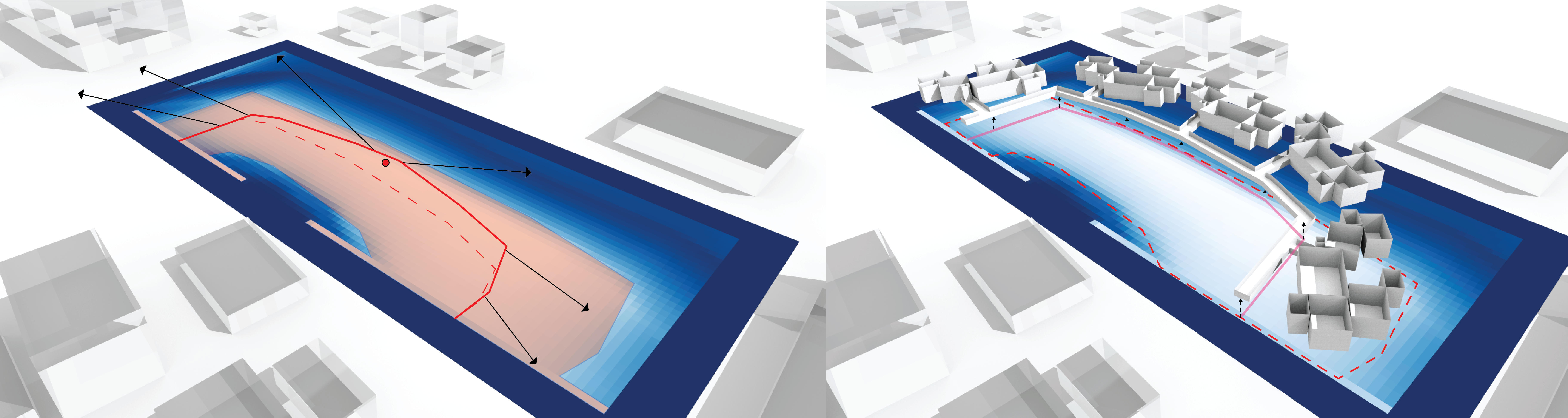
Post processing

The raw predicted data, as described before is a fuzzy shape. Hence a corridor must be inferred out of the same. The process of creating the corridor from the raw prediction is as follows:

• A cut-off value of fitness is decided by the user to create a distinct shape - the red boundary
• The centerline of that shape is then determined - dashed line
• The centerline is then stretched to make one of the extremes, cross beyond the centroid.
• Black Lines extending away from the centerline would be the connectors along which the units would be simulated using the physics engine, which is used to generate the final floor plan.

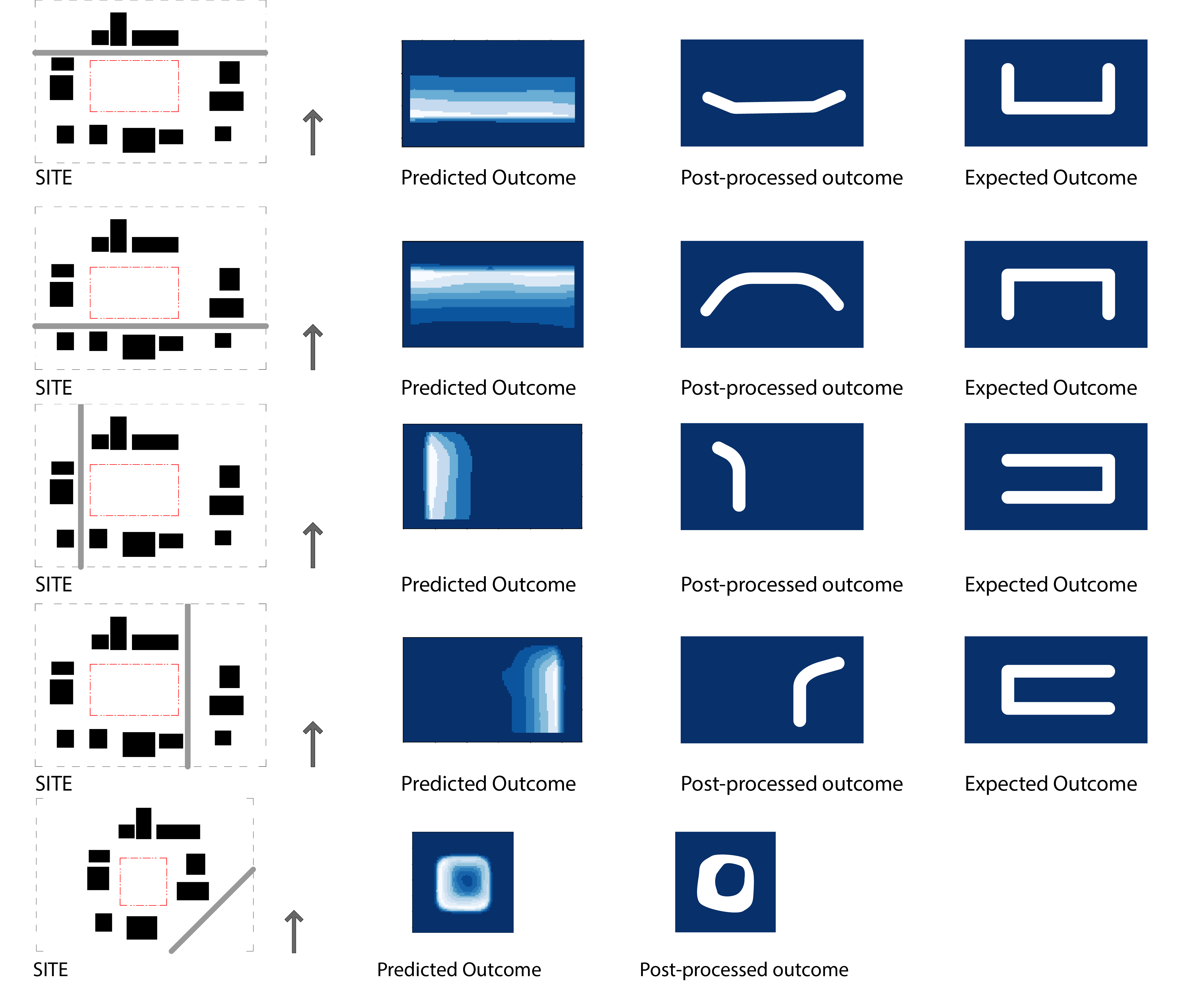
Predicted outcomes

Some notes and examples of what came out of this exercise

• The result of the two implicit goals - “U-shaped floor plan facing the road and the longer northern façade” shows that the model has been able to emulate partially.
• The post processed result clearly shows a result where one of the two implicit goals are met. Only the U-shaped floor plan facing the road is seen to be accommodated. A more balanced dataset would probably result in a more holistic ‘understanding’ on the part of the neural network.
• This last case was to test the limits of the neural network. There weren’t any roads at an angle to the site in the dataset. Yet the network predicts an acceptable outcome.

Future expandability

Below is an example of a completed simulation. Here for the sake of demonstration the site has been evaluated at multiple levels and the corresponding predictions have been made at different levels

• In the framework demonstrated, the inputs fed in are the cumulative solar data, the distance from the site edge and the distance from the adjacent road.
• An interesting question arises, what if we were to input in other pieces of site data such as terrain or view corridors? How complex can the framework get before it would break?